News and Blog Articles

Recently we wrote about the great benefit of control accounts where a balance is changing across a model – setting out calculations row by row, totalling up the result for the period and carrying it forward so that the closing balance for the last period becomes the opening balance for the current period.

It’s not just balance sheet line items that are candidates for calculation via control accounts.  Any calculation where you have a balance changing across time becomes a candidate for a control account.  That could be something ‘financial’ or something operational/ non-financial.

We’ve seen control accounts used for calculating recurring contract revenue (where you have new customers arriving, staying for a period of time, and then perhaps leaving via a forecast ‘churn rate’).  We’ve seen control accounts used to help calculate cash flow ‘waterfalls’ (cash available for debt repayment, cash applied to debt repayment become movements in the control account).  Also store roll outs where adding a new store results in a phased increase in revenue, costs and profit.

But we’ve also seen control accounts used to clarify operational balances as part of processes (where materials input into a process, wastage, usage are the movements), which results in calculations for volumes in the model themselves affecting financial figures.

Anything that you recognise as having the nature of a ‘balance’ changing from one period to another across your model becomes a candidate for treatment via a control account.

Straight line depreciation is easy to describe (“We’re going to write off new assets in a straight line over an input number of years e.g. £100 over 5 years = £20 of depreciation each year) but potentially becomes difficult to model, depending on how you decide to tackle it.

If you’re not careful you could end up replicating your company’s fixed asset schedule, layering in every asset (together with its depreciation schedule).  That’s probably more detail than you need for a forward-looking forecast that you want to be able to flex easily to explore ‘what if’ scenarios.

You need some kind of sensible simplification for straight line depreciation.  But it’s never going to be super-simple, given that you’ve got new assets arriving regularly, each needed to be depreciated for a number of years from the point it arrives.  In the modelling what we’re trying to do is avoid a situation where you have to set all the detail out in big tables in the model that could become hard to flex.  What we’re looking for is some kind of helpful simplification.

Let’s have a think about the £100 asset mentioned as an example earlier.  It’s going to be depreciated over 5 years = £20 a year.  When the asset ‘lands’ the depreciation expense is going to go up by £20 a year.  Then the expense is going to run at that £20 per year.  At the end of the 5 years, with the asset written down to zero, the £20 regular depreciation expense is going to end/ finish.

Do you see how you could start to look at the depreciation expense itself as a candidate for modelling via a control account?  £20 in at the start, running for 5 years, then removed at the end.

The benefit to the compact control account for modelling the depreciation expense is that it allows us room to add a next asset in a subsequent period (the new asset will start to add to our running total for the depreciation expense, until it is fully depreciated) and so on.

It’s probably best if we illustrate the approach by looking at an example.

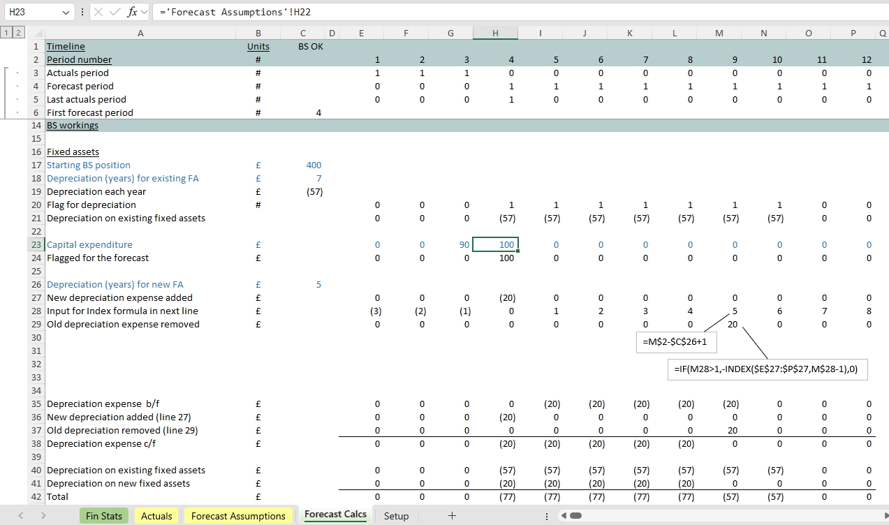
In the example below you can see a new asset of £100 arriving in period 4 column H of the model – see cell H23.

The depreciation associated with that asset is easily calculated – it’s £100/ the 5 years in C26.  You can see the £20 depreciation expense calculated in cell H27.

Now let’s take a look at the control account for this.  The new £20 expense arrives in the control account at H36.  It runs for 5 years before it is removed in cell M37.  The depreciation expense runs for 5 years at £20 each year as expected (row 38).

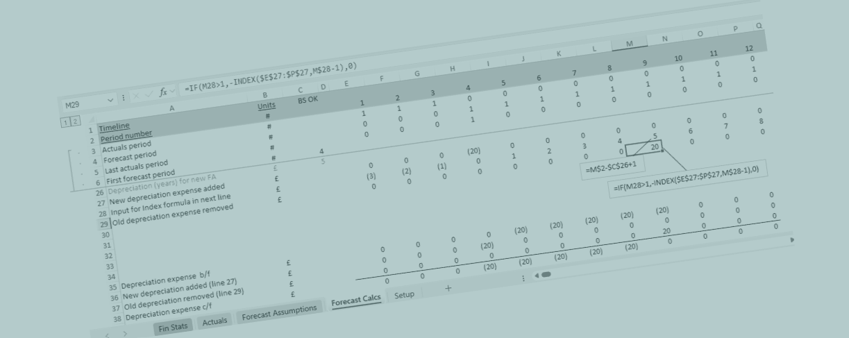
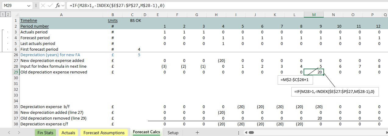
To turn the depreciation expense off in column M we’ve made use of the formula at line 29.  It ‘bumps’ the depreciation expense to the right by 5 periods, so it can be used in column M to turn depreciation off.  You might ordinarily gravitate to Excel’s Offset function for moving figures to the right.  However, because Offset is ‘volatile’, we’ve decided to use Index as the alternative for that job.

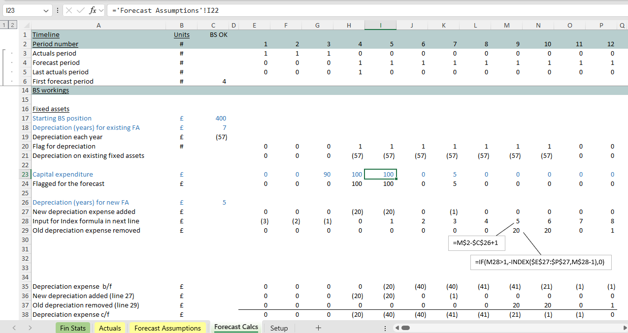
Let’s have a look at what happens when we test by adding new assets.  If we add a second £100 asset in period 5 column I, we can see an extra £20 depreciation expense arriving at row 38.   If we add an asset in period 7 column K the new depreciation expense associated with that asset arrives too.  It works!

If you’ve tried to model this yourself a different way, perhaps you’re appreciating the functionality and flexibility we’ve got here.  We can layer in any new value at any time, and the control account helps us calculate the costs associated with that.

 Perhaps you’re also now appreciating the power of control accounts/ corkscrews beyond their most common application (in modelling balance sheet line items in financial statements).  They enable us to flexibly ‘layer up’ models (new customers, new stores, new volumes of materials) and keep a clear running total of the revenues or costs associated with those new layers.

That means that anything you start to recognise as a ‘balance’ with movements attached becomes a candidate for the clarity that modelling via a control account/ corkscrew provides.

Control accounts (where you realise you can use them) really are a wonderful technique for keeping model calculations as simple and clear as possible, and an essential tool in running some of the trickiest calculations you’ll encounter in financial modelling.